
 Python Tutorials Python Tutorials | (back to the list of tutorials) |
 Mathematics of NURBS Geometry

Similarly, a NURBS surface is defined by the formula below, where now control points Pi,j and weights wi,j are provided as n x m matrix. This is a function of two parameters u and v and it returns spatial coordinates corresponding to the input u and v.

For more detail description of NURBS geometries and basis functions, see Wikipedia pages of NURBS, B-Spline and Bernstein Polynomial
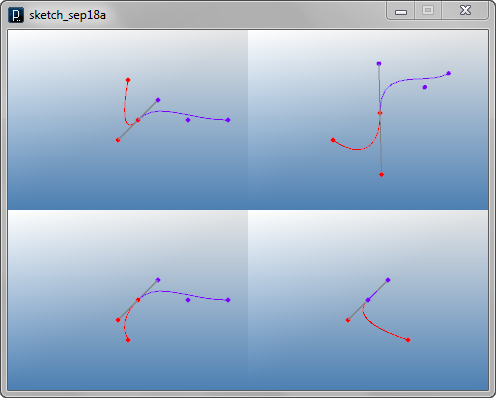
Creating NURBS Curves and Surfaces![]()
![]()
![]()
![]()
add_library('igeo')

size( 480, 360, IG.GL )

controlPoints1 = []
controlPoints1.append( IVec(0, 0, 0) )
controlPoints1.append( IVec(20, 30, 30) )
controlPoints1.append( IVec(40, -30, -30) )
controlPoints1.append( IVec(60, 0, 0) )

deg1 = 3
ICurve(controlPoints1, deg1).clr(0)

controlPoints2 = []
controlPoints2.append( IVec4(0, 0, 0, 1) )
controlPoints2.append( IVec4(20, 30, 30, 0.5) )
controlPoints2.append( IVec4(40, -30, -30, 0.5) )
controlPoints2.append( IVec4(60, 0, 0, 1) )

deg2 = 3
ICurve(controlPoints2, deg2).clr(1.,0,0)

controlPoints3 = [ \
  [ IVec(-70,0,0), IVec(-70,20,30), IVec(-70,40,0) ], \
  [ IVec(-50,30,30), IVec(-50,50,60), IVec(-50,70,30) ], \
  [ IVec(-30,-30,-30), IVec(-30,-10,0), IVec(-30,10,-30) ], \
  [ IVec(-10,0,30), IVec(-10,20,60), IVec(-10,40,30) ] ]

udeg3 = 3
vdeg3 = 2
ISurface(controlPoints3, udeg3, vdeg3).clr(0)

controlPoints4 = [ \
  [ IVec4(-70,0,0,1), IVec4(-70,20,30,.5), IVec4(-70,40,0,1) ], \
  [ IVec4(-50,30,30,.5), IVec4(-50,50,60,.5), IVec4(-50,70,30,.5) ], \
  [ IVec4(-30,-30,-30,.5), IVec4(-30,-10,0,.5), IVec4(-30,10,-30,.5) ], \
  [ IVec4(-10,0,30,1), IVec4(-10,20,60,.5), IVec4(-10,40,30,1) ] ]

udeg4 = 3
vdeg4 = 2
ISurface(controlPoints4, udeg4, vdeg4).clr(1,.5,1)

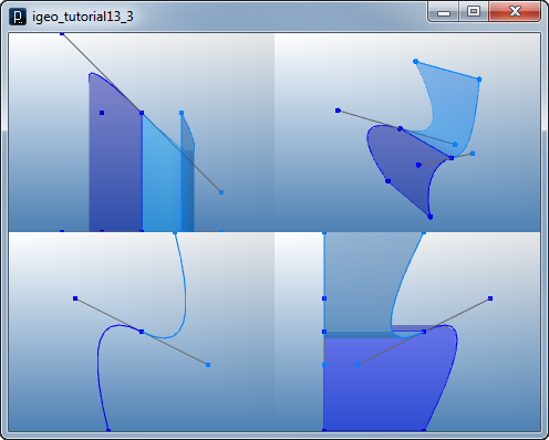
Continuity of NURBS Geometry![]()
![]()
![]()
![]()
add_library('igeo')

size( 480, 360, IG.GL )

curveEdgePt = IVec(10,0,0)
curveTangent = IVec(20,20,20)

cpts1 = []
cpts1.append( curveEdgePt )
cpts1.append( curveEdgePt.dup().sub(curveTangent) )
cpts1.append( IVec(0, 40, -40) )

cpts2 = []
cpts2.append( curveEdgePt )
cpts2.append( curveEdgePt.dup().add(curveTangent) )
cpts2.append( IVec(60,0,0) )
cpts2.append( IVec(100,0,0) )

ICurve(cpts1, 2).clr(1.,0,0)
ICurve(cpts2, 3).clr(.5,0,1)

# showing control points
for pt in cpts1 :
    IPoint(pt).clr(1.,0,0)

for pt in cpts2 :
    IPoint(pt).clr(.5,0,1)

# showing straight relationship
ICurve(cpts1[1], cpts2[1])
![]()
![]()
![]()
![]()
add_library('igeo')

size( 480, 360, IG.GL )

surfaceTangent1 = IVec(20, 0, -10)
surfaceTangent2 = IVec(20, -20, -10)
surfaceEdgePt1 = IVec(0, 0, 0)
surfaceEdgePt2 = IVec(0, 30, 0)

cpts3 = []
cpts3.append([])
cpts3[0].append(surfaceEdgePt1)
cpts3[0].append(surfaceEdgePt2)
cpts3.append([])
cpts3[1].append(surfaceEdgePt1.dup().sub(surfaceTangent1))
cpts3[1].append(surfaceEdgePt2.dup().sub(surfaceTangent2))
cpts3.append([])
cpts3[2].append(IVec(-10, 0, -30))
cpts3[2].append(IVec(-10, 30, -30))

cpts4 = []
cpts4.append([])
cpts4[0].append(surfaceEdgePt1)
cpts4[0].append(surfaceEdgePt2)
cpts4.append([])
cpts4[1].append(surfaceEdgePt1.dup().add(surfaceTangent1))
cpts4[1].append(surfaceEdgePt2.dup().add(surfaceTangent2))
cpts4.append([])
cpts4[2].append(IVec(10, 0, 30))
cpts4[2].append(IVec(10, 30, 30))

ISurface(cpts3, 2, 1).clr(0,0,1.)
ISurface(cpts4, 2, 1).clr(0,.5,1.)

# showing control points
for pts in cpts3 :
    for pt in pts :
        IPoint(pt).clr(0,0,1.)

for pts in cpts4 :
    for pt in pts :
        IPoint(pt).clr(0,.5,1.)

# showing straight relationship
ICurve(cpts3[1][0], cpts4[1][0])
ICurve(cpts3[1][1], cpts4[1][1])
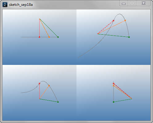
Point on NURBS Curve![]()
![]()
![]()
![]()
add_library('igeo')

size( 480, 360, IG.GL )

cpts = [ IVec(-60,0,0), IVec(-20,0,0), IVec(20,0,60), IVec(60,0,-30) ]

curve = ICurve(cpts, 2)

pt1 = curve.pt(0.5)
pt2 = curve.pt(0.8)
pt3 = curve.pt(1.0)

# showing points
IPoint(pt1).clr(1.,0,0)
IPoint(pt2).clr(1.,.5,0)
IPoint(pt3).clr(0,.5,0)

# using them for creating other geometries
ICurve(IVec(0,60,-20), pt1).clr(1.,0,0)
ICurve(IVec(0,60,-20), pt2).clr(1.,.5,0)
ICurve(IVec(0,60,-20), pt3).clr(0,.5,0)
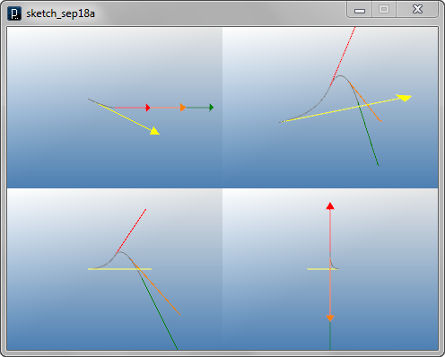
Tangent on NURBS Curve![]()
![]()
![]()
![]()
add_library('igeo')

size( 480, 360, IG.GL )

cpts = [ IVec(-30,10,0), IVec(-10,0,0), IVec(10,0,30), IVec(30,0,-10) ]

curve = ICurve(cpts, 2)

tan1 = curve.tan(0)
tan2 = curve.tan(0.5)
tan3 = curve.tan(0.8)
tan4 = curve.tan(1.0)

# showing arrows at each point on the curve
tan1.show(curve.pt(0)).clr(1.,1.,0).size(10)
tan2.show(curve.pt(0.5)).clr(1.,0,0).size(10)
tan3.show(curve.pt(0.8)).clr(1,.5,0).size(10)
tan4.show(curve.pt(1.0)).clr(0,.5,0).size(10)
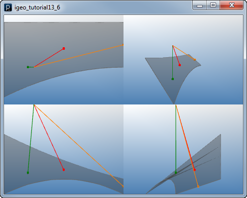
Point on NURBS Surface![]()
![]()
![]()
![]()
add_library('igeo')

size( 480, 360, IG.GL )

cpts = [[ IVec(-40,-20,-20), IVec(0,0,0), IVec(40,0,-20) ], \
        [ IVec(-40,30,20), IVec(0,30,0), IVec(40,30,-10) ]]

surface = ISurface(cpts,1,2)

pt1 = surface.pt(0.5,0.5)
pt2 = surface.pt(0.5,1.0)
pt3 = surface.pt(0.3,0.2)

# showing points
IPoint(pt1).clr(1.,0,0)
IPoint(pt2).clr(1,.5,0)
IPoint(pt3).clr(0,.5,0)

# using them for creating other geometries
ICurve(IVec(-20,0,40), pt1).clr(1.,0,0)
ICurve(IVec(-20,0,40), pt2).clr(1,.5,0)
ICurve(IVec(-20,0,40), pt3).clr(0,.5,0)
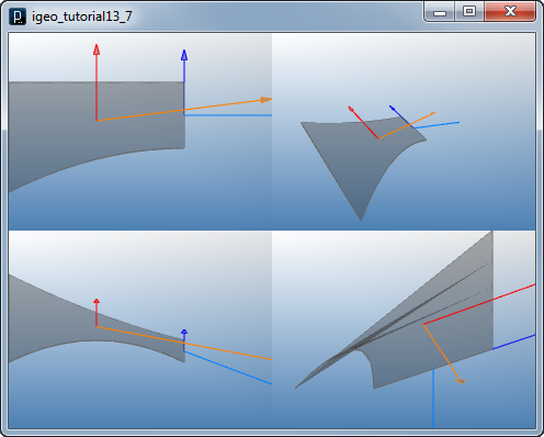
Tangent on NURBS Surface![]()
![]()
![]()
![]()
add_library('igeo')

size( 480, 360, IG.GL )

cpts = [[ IVec(-40,-20,-20), IVec(0,0,0), IVec(40,0,-20) ], \
        [ IVec(-40,30,20), IVec(0,30,0), IVec(40,30,-10) ]]

surface = ISurface(cpts,1,2)

utan1 = surface.utan(0.5,0.5)
utan2 = surface.utan(0.5,1.0)
vtan1 = surface.vtan(0.5,0.5)
vtan2 = surface.vtan(0.5,1.0)

# showing arrows at each point on the surface
utan1.show(surface.pt(0.5,0.5)).clr(1.,0,0).size(5)
utan2.show(surface.pt(0.5,1.0)).clr(0,0,1.).size(5)
vtan1.show(surface.pt(0.5,0.5)).clr(1,.5,0).size(5)
vtan2.show(surface.pt(0.5,1.0)).clr(0,.5,1).size(5)
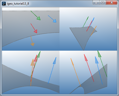
Normal on NURBS Surface![]()
![]()
![]()
![]()
add_library('igeo')

size( 480, 360, IG.GL )

cpts = [[ IVec(-40,30,20), IVec(0,30,0), IVec(40,30,-10) ], \
        [ IVec(-40,-20,-20), IVec(0,0,0), IVec(40,0,-20) ]]

surface = ISurface(cpts,1,2)

normal1 = surface.nml(0.5,0.5).len(40)
normal2 = surface.nml(1.0,0.5).len(40)
normal3 = surface.nml(0.0,0.5).len(40)
normal4 = surface.nml(0.2,0.8).len(40)

# showing arrows at each point on the surface
normal1.show(surface.pt(0.5,0.5)).clr(1.,0,0).size(10)
normal2.show(surface.pt(1.0,0.5)).clr(1.,.5,0).size(10)
normal3.show(surface.pt(0.0,0.5)).clr(0,.5,0).size(10)
normal4.show(surface.pt(0.2,0.8)).clr(0,.5,1).size(10)
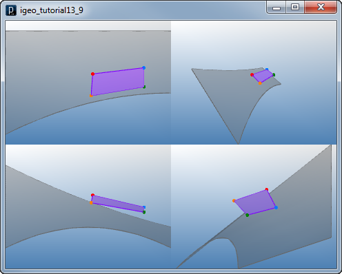
Offset Point on NURBS Surface![]()
![]()
![]()
![]()
add_library('igeo')

size( 480, 360, IG.GL )

cpts = [[ IVec(-40,30,20), IVec(0,30,0), IVec(40,30,-10) ], \
        [ IVec(-40,-20,-20), IVec(0,0,0), IVec(40,0,-20) ]]

surface = ISurface(cpts,1,2)

pt1 = surface.pt(0.5, 0.5, 10)
pt2 = surface.pt(0.8, 0.5, 10)
pt3 = surface.pt(0.8, 0.8, 10)
pt4 = surface.pt(0.5, 0.8, 10)

# showing points
IPoint(pt1).clr(1.,0,0)
IPoint(pt2).clr(1.,.5,0)
IPoint(pt3).clr(0,.5,0)
IPoint(pt4).clr(0,.5,1)

# using them for creating other geometries
ISurface(pt1,pt2,pt3,pt4).clr(.5,0,1)
HOME
FOR PROCESSING
DOWNLOAD
DOCUMENTS
TUTORIALS (Java /
Python)
GALLERY
SOURCE CODE(GitHub)
PRIVACY POLICY
ABOUT/CONTACT
