
 Python Tutorials Python Tutorials | (back to the list of tutorials) |
 Simple Field: Gravity and Attractor
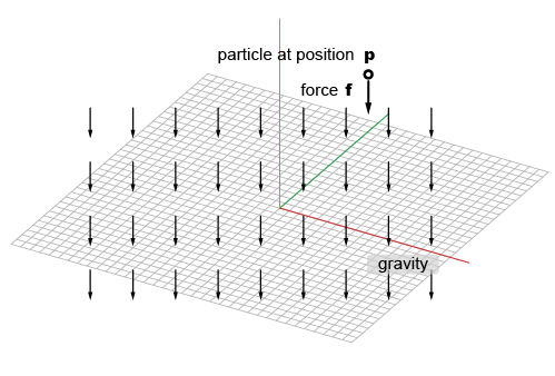
An attractor and a repulsion force defines a 3D vector force towards the position of attractor/repulsion from the position of a particle.

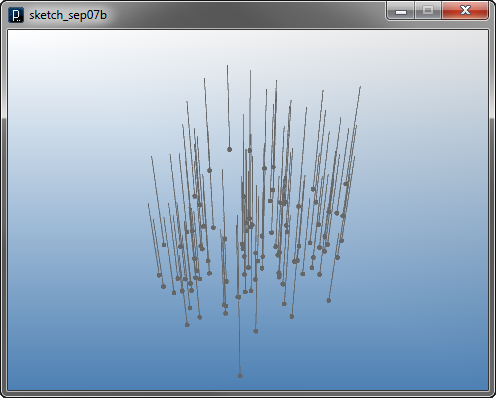
Besides creating gravity and a attractor in previous example codes, iGeo library has a class of gravity, IGravity and a class of attractor IAttractor as a type of generic fields. The example below shows a code to use IGravity class. You can specify the gravity vector by x, y and z in the constructor. This code also use a type of a particle class IParticleTrajectory, which creates trajectory lines of the particle.
![]()
![]()
![]()
![]()
add_library('igeo')

size(480, 360, IG.GL)
IG.duration(50)
IGravity(0,0,-10) # direction and intensity of gravity

for i in range(100) :
    IParticleTrajectory(IRand.pt(-100,100));# random points from (-100,-100,-100) to (100,100,100)
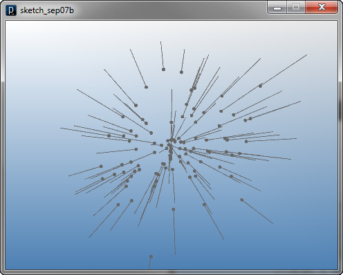
The code below is an example of IAttractor. You can specify the position of attractor in the constructor and the intensity of the attractor by intensity(double) method. If you put negative number in the intensity, it provides a repulsion force instead of an attraction force.
![]()
![]()
![]()
![]()
add_library('igeo')

size(480, 360, IG.GL)
IG.duration(100)
IAttractor(0,0,0).intensity(10) # attractor at (0,0,0) with intensity 10

for i in range(100) :
    IParticleTrajectory(IRand.pt(-100,100))# random points from (-100,-100,-100) to (100,100,100)
Visualizing Field
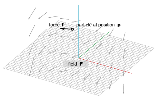

Because the output vectors can vary at different positions, you'd want to sample the output at many positions to comprehend the whole field. iGeo library has a class of IFieldVisualizer to have a 3D matrix of sampled vectors to visualize fields. To use IFieldVisualizer, you specify x, y, z coordinates of two corners for a 3D matrix to sample vectors. As default it creates 10x10x10 matrix within the specified bounding box.
![]()
![]()
![]()
![]()
add_library('igeo')

size(480, 360, IG.GL)

IAttractor(-50,0,0).intensity(10).clr(1.0,0,0) #attractor
IAttractor(50,0,0).intensity(-10).clr(0,0,1.0) #repulsion

# creating 3D matrix. default is 10x10x10.
# input argument is (minX, minY, minZ, maxX, maxY, maxZ)
IFieldVisualizer(-100,-100,-100,100,100,100)
You can show only 2D vector field by putting same z coordinates for the bounding box and specifying sample number in z to be 1.
![]()
![]()
![]()
![]()
add_library('igeo')

size(480, 360, IG.GL)

IAttractor(-50,0,0).intensity(10).clr(1.0,0,0) #attractor
IAttractor(50,0,0).intensity(-10).clr(0,0,1.0) #repulsion

# last 3 inputs are sample number in x, y, z.
IFieldVisualizer(-100, -50, 0, 100, 50, 0, 40, 20, 1)
You can also change min/max colors to show the intensity by the method colorRange(min red, min green, min blue, max red, max green, max blue). Although the length of sampled vector is all same as default, you can change it to be proportional to the intensity of the field by putting false to the method fixLength(boolean).
![]()
![]()
![]()
![]()
add_library('igeo')

size(480, 360, IG.GL)

IAttractor(-50,0,0).intensity(10).clr(1.0,0,0) #attractor
IAttractor(50,0,0).intensity(-10).clr(0,0,1.0) #repulsion

visualizer = IFieldVisualizer(-100,-50,0,100,50,0,40,20,1)

# color of min/max intensty. inputs are (min red, green, blue, max red, green, blue)
visualizer.colorRange(0.0,0.0,0.0, 0.0,1.0,0.)

# use variable length; now length is proportioanl to the intensity
visualizer.fixLength(false)

Decay of Field from Defining GeometryNo decay provides constant intensity. This is a default decay type of most of fields class in the library. You can also specify this type by noDecay() method.

![]()
![]()
![]()
![]()
add_library('igeo')

size(480, 360, IG.GL)

IAttractor(0,0,0).noDecay()

IFieldVisualizer(-100,-100,0,100,100,0,20,20,1).fixLength(False)

The second decay type is linear decay. This type is specified with a parameter of threshold. When the distance from the geometry is equal to the threshold, the intensity becomes zero. You can specify this type by linearDecay(threshold). There is also an alias of this method linear(threshold).

![]()
![]()
![]()
![]()
add_library('igeo')

size(480, 360, IG.GL)

IAttractor(0,0,0).linearDecay(100)

IFieldVisualizer(-100,-100,0,100,100,0,20,20,1).fixLength(False)

The third decay type is Gaussian decay. This type is specified with a parameter of threshold as well. The intensity follows the Gaussian function and the threshold is equal to double of the standard deviation. Even when the distance is larger than the threshold, the intensity doesn't become zero but gradually gets closer to zero. You can specify this type by gaussianDecay(threshold). There is also an alias of this method gaussian(threshold).

![]()
![]()
![]()
![]()
add_library('igeo')

size(480, 360, IG.GL)

IAttractor(0,0,0).gaussianDecay(100)

IFieldVisualizer(-100,-100,0,100,100,0,20,20,1).fixLength(False)
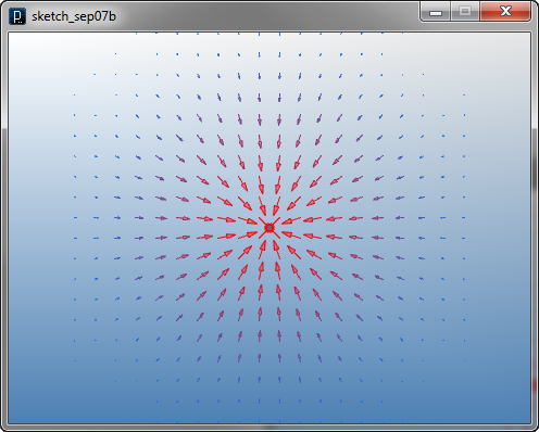
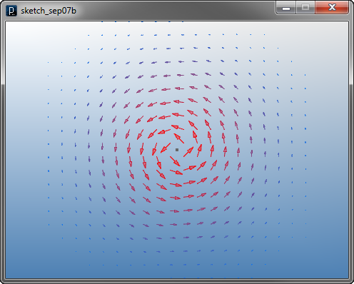
Field Defined by Points ![]()
![]()
![]()
![]()
add_library('igeo')

size(480, 360, IG.GL)

IPointCurlField(IVec(0,0,0),IVec(0,0,1)).gaussianDecay(100)

IFieldVisualizer(-100,-100,0,100,100,0,20,20,1).fixLength(False)
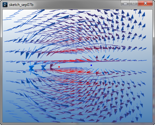
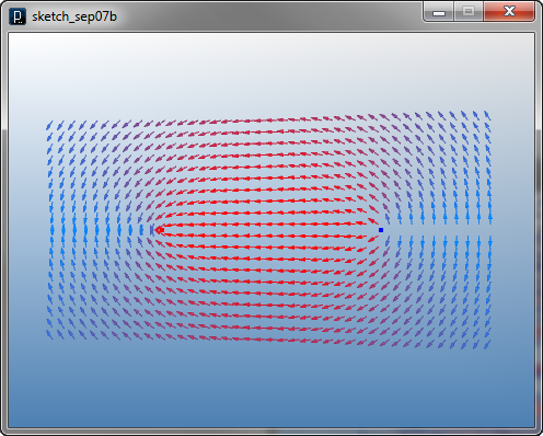
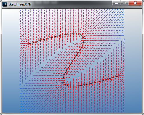
Field Defined by Curves (Attractor, Tangent, Curl)First, a curve attractor field attracts a particle to the closest point on the curve. The class in the library is ICurveAttractorField. You put one curve as an input to build the curve attractor. The curve attractor field is visualized below.
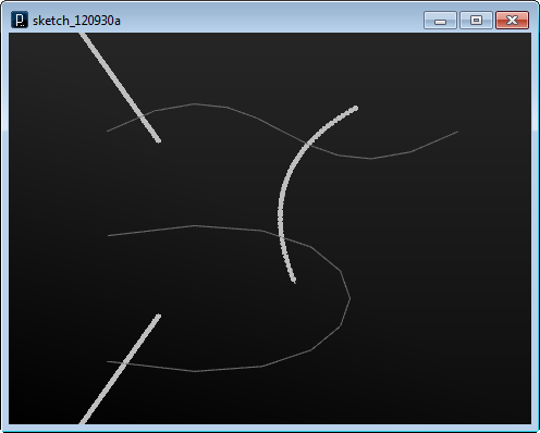
The sample input file used below is this file.
curve_field1.3dm
![]()
![]()
![]()
![]()
add_library('igeo')

size(480, 360, IG.GL)

IG.open("curve_field1.3dm")

for i in range(IG.curveNum()) :
    ICurveAttractorField(IG.curve(i)).intensity(10).linear(50)

IFieldVisualizer(-20,-20,0, 20,20,0, 40,40,1)
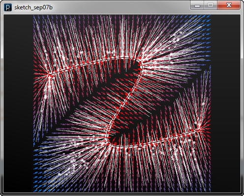
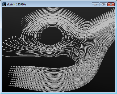
The code below shows the response of particles to the curve attractor fields with trajectory lines.
![]()
![]()
![]()
![]()
add_library('igeo')

size(480, 360, IG.GL)

IG.darkBG()
IG.open("curve_field1.3dm")

for i in range(IG.curveNum()) :
    ICurveAttractorField(IG.curve(i)).intensity(10).linear(50)

IFieldVisualizer(-20,-20,0, 20,20,0, 40,40,1)

for i in range(1000) :
    IParticleTrajectory(IRand.pt(-20,-20,20,20)).fric(0.1).clr(1.0,0.7)
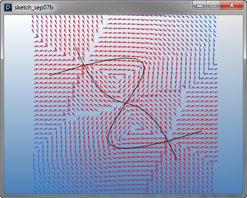
The second curve field is a curve tangent field. This field defines a force towards the direction of a tangent vector of the curve at the closest point from the given particle position. The class of this type of field is ICurveTangentField. The field is visualized below.
![]()
![]()
![]()
![]()
add_library('igeo')

size(480, 360, IG.GL)

IG.open("curve_field1.3dm")

for i in range(IG.curveNum()) :
    ICurveTangentField(IG.curve(i)).intensity(10).linear(50)

IFieldVisualizer(-20,-20,0, 20,20,0, 40,40,1)

The below example is to show the response of particles to the field.
![]()
![]()
![]()
![]()
add_library('igeo')

size(480, 360, IG.GL)

IG.darkBG()
IG.open("curve_field1.3dm")

for i in range(IG.curveNum()) :
    ICurveTangentField(IG.curve(i)).intensity(10).linear(50)

IFieldVisualizer(-20,-20,0, 20,20,0, 40,40,1)

for i in range(1000) :
    IParticleTrajectory(IRand.pt(-20,-20,20,20)).fric(0.1).clr(1.0,0.7)

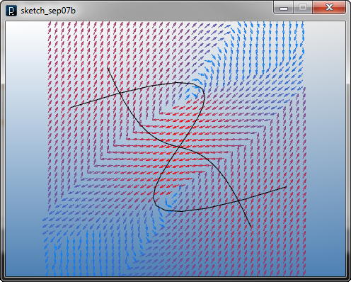
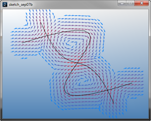
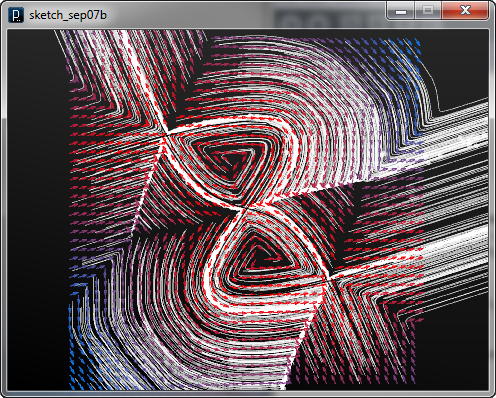
The third curve field is a curve curl field. This defines a force by a cross vector of a tangent vector on the curve and the difference vector from the closest point on the curve to the given position of a particle. As result, the force is always perpendicular to the tangent and the particle shows a curling behavior. The class of this field is ICurveCurlField. The below shows visualization of the field.
![]()
![]()
![]()
![]()
add_library('igeo')

size(480, 360, IG.GL)

IG.open("curve_field1.3dm")

for i in range(IG.curveNum()) :
    ICurveCurlField(IG.curve(i)).intensity(10).linear(50)

IFieldVisualizer(-20,-20,-1, 20,20,1, 40,40,2)

The example blow shows the response of particles to the field.
![]()
![]()
![]()
![]()
add_library('igeo')

size(480, 360, IG.GL)

IG.darkBG()
IG.open("curve_field1.3dm")

for i in range(IG.curveNum()) :
    ICurveCurlField(IG.curve(i)).intensity(10).linear(50)

IFieldVisualizer(-20,-20,-1, 20,20,1, 40,40,2)

for i in range(1000) :
    IParticleTrajectory(IRand.pt(-20,-20,20,20)).fric(0.1).clr(1.0,0.7)
Multiple Summed Fields
The sample input file of multiple curves used below is this file.
curve_field2.3dm
![]()
![]()
![]()
![]()
add_library('igeo')

size(480, 360, IG.GL)

IG.open("curve_field2.3dm")

for i range(IG.curveNum()) :
    ICurveTangentField(IG.curve(i)).intensity(10).linear(50)

IFieldVisualizer(-20,-20,0, 20,20,0, 40,40,1)
![]()
![]()
![]()
![]()
add_library('igeo')

size(480, 360, IG.GL)

IG.darkBG()
IG.open("curve_field2.3dm")

for i in range(IG.curveNum()) :
    ICurveTangentField(IG.curve(i)).intensity(10).linear(50)

IFieldVisualizer(-20,-20,0, 20,20,0, 40,40,1)

for i in range(1000) :
    IParticleTrajectory(IRand.pt(-20,-20,20,20)).fric(0.1).clr(1.0,0.7)

Vector summation of multiple fields sometimes changes the behavior drastically especially when fields have no decay, because some local area responding to an adjacent source curve is equally influenced by other source curves in farther location. Another pair of examples below shows when you limit the influence by putting a smaller threshold.
![]()
![]()
![]()
![]()
add_library('igeo')

size(480, 360, IG.GL)

IG.open("curve_field2.3dm")

for i in range(IG.curveNum()) :
    ICurveTangentField(IG.curve(i)).linear(5).intensity(10)

IFieldVisualizer(-20,-20,0, 20,20,0, 40,40,1)
![]()
![]()
![]()
![]()
add_library('igeo')

size(480, 360, IG.GL)

IG.darkBG()
IG.open("curve_field2.3dm")

for i in range(IG.curveNum()) :
    ICurveTangentField(IG.curve(i)).linear(5).intensity(10)

IFieldVisualizer(-20,-20,0, 20,20,0, 40,40,1)

for i in range(1000) :
    IParticleTrajectory(IRand.pt(-20,-20,20,20)).fric(0.1).clr(1.0,0.7)

Compound Field The code below is a example of a compound field. To add a field as a member of compound field, you use add( field ).
![]()
![]()
![]()
![]()
add_library('igeo')

size(480, 360, IG.GL)
IG.open("curve_field2.3dm")

field = ICompoundField()
for i in range(IG.curveNum()) :
    field.add(ICurveTangentField(IG.curve(i)).linear(50).intensity(10))

IFieldVisualizer(-20,-20,0, 20,20,0, 40,40,1)
![]()
![]()
![]()
![]()
add_library('igeo')

size(480, 360, IG.GL)

IG.darkBG()
IG.open("curve_field2.3dm")

field = ICompoundField()
for i in range(IG.curveNum()) :
    field.add(ICurveTangentField(IG.curve(i)).linear(50).intensity(10))

IFieldVisualizer(-20,-20,0, 20,20,0, 40,40,1)

for i in range(1000) :
    IParticleTrajectory(IRand.pt(-20,-20,20,20)).fric(0.1).clr(1.0,0.7)
A gravity field doesn't have a source geometry as mentioned above because
gravity generates a constant force everywhere.
However, you can specify a point as a source geometry to create
a compound field. If you feed
a position vector and the gravity direction vector to
the constructor
The code below shows an example of construction of a compound field out of multiple gravity fields.
![]()
![]()
![]()
![]()
add_library('igeo')

size(480, 360, IG.GL)

field = ICompoundField()
for i in range(30) :
    dir = IRand.pt(-1,-1,1,1)
    pos = IRand.pt(-20,-20,20,20)
    field.add(IGravity(pos, dir))

IFieldVisualizer(-20,-20,0, 20,20,0, 40,40,1)

![]()
![]()
![]()
![]()
add_library('igeo')

size(480, 360, IG.GL)

IG.darkBG()

field = ICompoundField()
for i in range(30) :
    dir = IRand.pt(-1,-1,1,1)
    pos = IRand.pt(-20,-20,20,20)
    field.add(IGravity(pos, dir))

IFieldVisualizer(-20,-20,0, 20,20,0, 40,40,1)

for i in range(2000) :
    IParticleTrajectory(IRand.pt(-20,-20,20,20)).fric(0.1).clr(1.0,0.7)
Another example of a compound field is with multiple IPointCurlField.
![]()
![]()
![]()
![]()
add_library('igeo')

size(480, 360, IG.GL)

IG.darkBG()

field = ICompoundField()
for i in range(30) :
    field.add(IPointCurlField(IRand.pt(-20,-20,20,20),IVec(0,0,1)).gaussian(10))

IFieldVisualizer(-20,-20,0, 20,20,0, 40,40,1)

for i in range(2000) :
    IParticleTrajectory(IRand.pt(-20,-20,20,20)).fric(0.1).clr(1.0,0.7)

Or you can mix different types of fields together randomly with a probability switch IRand.pct(percent).
![]()
![]()
![]()
![]()
add_library('igeo')

size(480, 360, IG.GL)

IG.darkBG()

field = ICompoundField()
for i in range(30) :
    if IRand.pct(40) :
        field.add(IAttractor(IRand.pt(-20,-20,20,20)).intensity(-10).gaussian(20))
    elif IRand.pct(50) :
        field.add(IPointCurlField(IRand.pt(-20,-20,20,20),IVec(0,0,1)))
    else :
        field.add(IGravity(IRand.pt(-20,-20,20,20),IRand.pt(-1,-1,1,1)))

IFieldVisualizer(-20,-20,0, 20,20,0, 40,40,1)

for i in range(2000) :
    IParticleTrajectory(IRand.pt(-20,-20,20,20)).fric(0.1).clr(1.0,0.7)

Field Defined by Surfaces (Tangent, Normal, Slope)The sample code below shows a surface tangent field of ISurfaceUTangentField. This field generates forces towards the U tangent vectors of the surface.
The sample surface file used below is this file.
surface_field1.3dm
![]()
![]()
![]()
![]()
add_library('igeo')

size(480, 360, IG.GL)
IG.open("surface_field1.3dm")

for i in range(IG.surfaceNum()) :
    ISurfaceUTangentField(IG.surface(i)).linear(50).intensity(10)

IFieldVisualizer(-20,-20,-2, 20,20,0, 20,20,2)
![]()
![]()
![]()
![]()
add_library('igeo')

size(480, 360, IG.GL)

IG.darkBG()
IG.open("surface_field1.3dm")

for i in range(IG.surfaceNum()) :
    ISurfaceUTangentField(IG.surface(i)).linear(50).intensity(10)

IFieldVisualizer(-20,-20,-2, 20,20,0, 20,20,2)

for i in range(1000) :
    IParticleTrajectory(IRand.pt(-20,-20,-5,20,20,0)).fric(0.1).clr(1.0,0.7)
The code below shows another surface tangent field in V direction using ISurfaceVTangentField class.
![]()
![]()
![]()
![]()
add_library('igeo')

size(480, 360, IG.GL)

IG.darkBG()
IG.open("surface_field1.3dm")

for i in range(IG.surfaceNum()) :
    ISurfaceVTangentField(IG.surface(i)).linear(50).intensity(10)

IFieldVisualizer(-20,-20,-2, 20,20,0, 20,20,2)

for i in range(1000) :
    IParticleTrajectory(IRand.pt(-20,-20,-5,20,20,0)).fric(0.1).clr(1.0,0.7)
The next surface field is a surface normal field of ISurfaceNormalField, which generates forces in the direction of surface normal vectors.
![]()
![]()
![]()
![]()
add_library('igeo')

size(480, 360, IG.GL)

IG.darkBG()
IG.open("surface_field1.3dm")

for i in range(IG.surfaceNum()) :
    ISurfaceNormalField(IG.surface(i)).linear(50).intensity(10)

IFieldVisualizer(-20,-20,-2, 20,20,0, 20,20,2)

for i in range(1000) :
    IParticleTrajectory(IRand.pt(-20,-20,-5,20,20,0)).fric(0.1).clr(1.0,0.7)

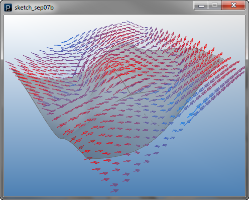
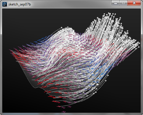
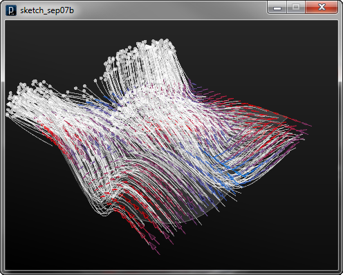
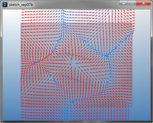
Another surface field is a surface slope field of I2DSurfaceSlopeField, which generates 2D vector only in XY direction (no force in Z direction) by the slope of a surface. If the surface has a valley in Z direction, that part acts as attractor and a hill causes a repulsion force.
![]()
![]()
![]()
![]()
add_library('igeo')

size(480, 360, IG.GL)

IG.open("surface_field1.3dm")

for i in range(IG.surfaceNum()) :
    I2DSurfaceSlopeField(IG.surface(i)).linear(50).intensity(10)

IFieldVisualizer(-20,-20,0, 20,20,0, 40,40,1)
![]()
![]()
![]()
![]()
add_library('igeo')

size(480, 360, IG.GL)

IG.darkBG()
IG.open("surface_field1.3dm")

for i in range(IG.surfaceNum()) :
    I2DSurfaceSlopeField(IG.surface(i)).linear(50).intensity(10)

IFieldVisualizer(-20,-20,0, 20,20,0, 40,40,1)

for i in range(2000) :
    IParticleTrajectory(IRand.pt(-20,-20,20,20)).fric(0.1).clr(1.0,0.7)

Initialize Particles with Points
The sample file of curves and points used below is this file.
curve_field_init1.3dm
![]()
![]()
![]()
![]()
add_library('igeo')

size(480, 360, IG.GL)

IG.darkBG()
IG.open("curve_field_init1.3dm")

fieldCurves = IG.layer("field").curves()
for crv in fieldCurves :
    ICurveTangentField(crv).linear(20).intensity(50)

points = IG.layer("particle").points()
for pt in points :
    IParticleTrajectory(pt).fric(0.2).clr(pt.clr())
    pt.del()
The following is the initial location of points specified in the rhino file.

Initialize Particles with Points on Curves
The sample file of curves used below is this file.
The curves for field and particle are stored in different layers.
curve_field_init2.3dm
![]()
![]()
![]()
![]()
add_library('igeo')

size(480, 360, IG.GL)

IG.darkBG()
IG.open("curve_field_init2.3dm")

fieldCurves = IG.layer("field").curves()
for crv in fieldCurves :
    ICurveTangentField(crv).linear(20).intensity(50)

divisionNum = 50;
particleCurves = IG.layer("particle").curves()
for crv in particleCurves :
    for j in range(divisionNum) :
        pos = crv.pt( 1.0/divisionNum*j )
        IParticleTrajectory(pos).fric(0.2).clr(crv.clr())

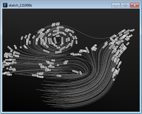
Initialize Particles with Surfaces and MeshesThe following is the example code to create particle (IParticleTrajectory) with input geometries in a specific layer in a input 3dm file. This code extracts instances of IGeometry from the specified layer in the internal server. IGeometry is a super class of IPoint, ICurve, ISurface, IMesh and IBrep. The method IG.geometries() or IG.layer(layerName).geometries() returns all geometries inside the internal server or inside the specified layer. The return value is an array containing any type of geometry and it can be mixture of different types if any.
The sample file of curves used below is this file.
curve_field_init3.3dm
![]()
![]()
![]()
![]()
add_library('igeo')

size(480, 360, IG.GL)
IG.duration(250)
IG.darkBG()
IG.open("curve_field_init3.3dm")

fieldCurves = IG.layer("field").curves()
for crv in fieldCurves :
    ICurveTangentField(crv).linear(20).intensity(50)

geometries = IG.layer("particle").geometries() # all geometries in "particle" layer
for geo in geometries :
    IParticleTrajectory([geo]).fric(0.2) # create a particle out of each geometry
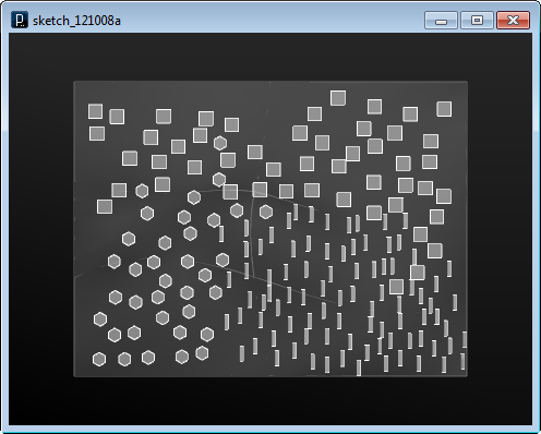
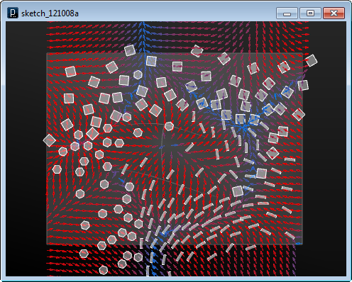
The image below shows the initial geometries from the input file.

Each input geometry is moved and rotated as a particle by the force field.
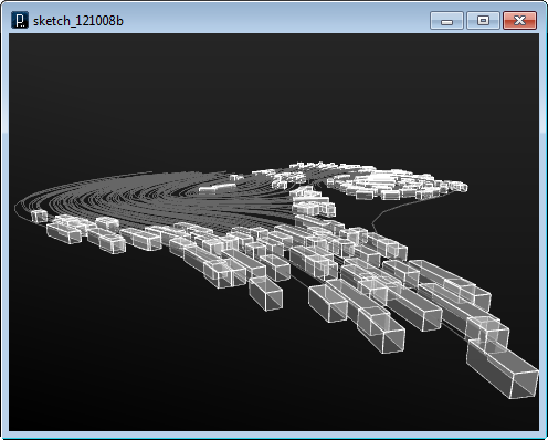
Another example below shows a code to convert input geometries into swarm agent (IBoid instance) to distribute geometries under the surface field condition and the swarming logic.
The sample file of curves used below is this file.
curve_field_init4.3dm
![]()
![]()
![]()
![]()
add_library('igeo')

size(480, 360, IG.GL)

IG.darkBG()
IG.duration(700)
IG.open("curve_field_init4.3dm")

fieldSurfaces = IG.layer("field").surfaces()
for srf in fieldSurfaces :
    I2DSurfaceSlopeField(srf).linear(50).intensity(10)

IFieldVisualizer(-20,-20,0, 20,20,0, 40,40,1)

geometries = IG.layer("particle").geometries()
for geo in geometries :
    b = IBoid([geo]).fric(0.2)
    b.cohesionRatio(5.0)
    b.cohesionDist(5.5)
    b.separationRatio(25.0)
    b.separationDist(5.0)
    b.alignmentRatio(15.0)
    b.alignmentDist(7.0)
Initial state.
Distribution under the surface field condition and the swarming logic. Geometries loosely gather around the valley areas of the field surface but keeping distance to other geometries by the swarm algorithm.
HOME
FOR PROCESSING
DOWNLOAD
DOCUMENTS
TUTORIALS (Java /
Python)
GALLERY
SOURCE CODE(GitHub)
PRIVACY POLICY
ABOUT/CONTACT
